C1_W2: Regression with Multiple Input Variables
This week, you’ll extend linear regression to handle multiple input features. You’ll also learn some methods for improving your model’s training and performance, such as vectorization, feature scaling, feature engineering and polynomial regression. At the end of the week, you’ll get to practice implementing linear regression in code.
C1_W2_M1 Multiple Linear Regression
C1_W2_M1_1 Multiple features
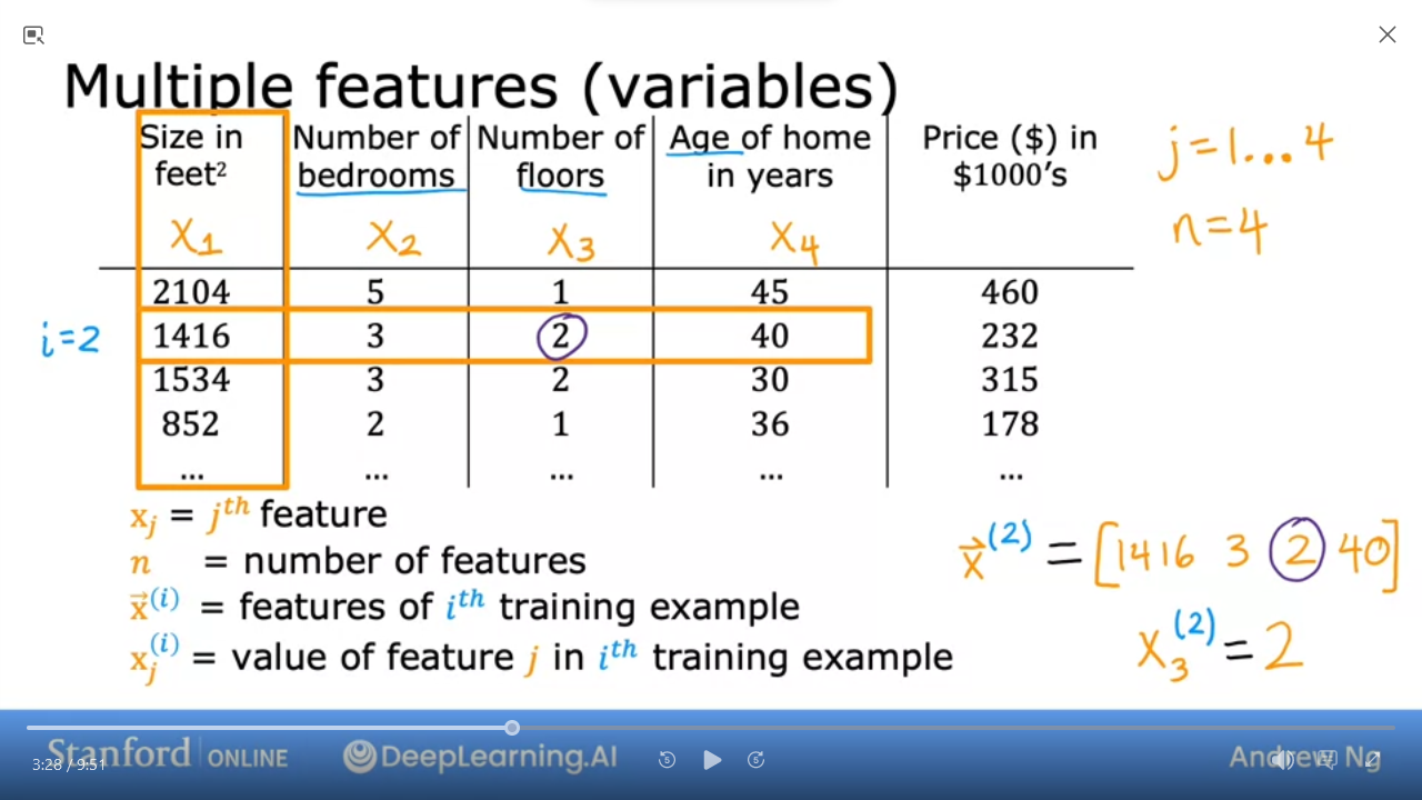 -$\vec{x}^{(i)}$= vector of 4 parameters for$i^{th}$row
=$[1416 3 2 40] $
-$\vec{x}^{(i)}$= vector of 4 parameters for$i^{th}$row
=$[1416 3 2 40] $
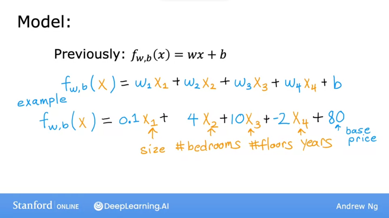
- In this example, house price increase by (multiply 1k)
-
0.1per square foot -
4per bedroom -
10per floor -
-2per year old - add
80base price
-
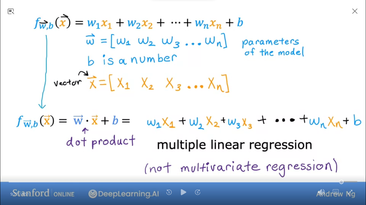
- We can simplify the model
- From linear algebra, this is a row vector as opposed to column vector
- this is multiple linear regression
- Not multivariate regression
Quiz
In the training set below (see slide: C1W2_M1_1 Multiple features), what is$x{1}^{(4)} $?
Ans
852C1_W2_M1_2 Vectorization part 1
Learning to write vectorized code allows you to take advantage of modern numberical linear algebra libraries, as well as maybe GPU hardware.
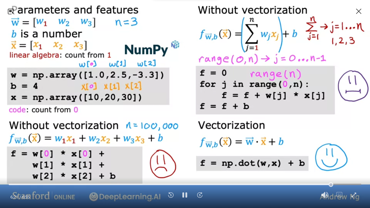
- Vector can be represented in Python as
np.array([1.0, 2.5, -3.3]) - if
nis large, this code (on left) is inefficient - for loop is more concise, but still not efficient
-
np.dot(w,x) + bis most efficient using vectorization - Vectorization has 2 benefits: concise and efficient
-
np.dotcan use parallel hardware
C1_W2_M1_3 Vectorization part 2
How does vectorized algorithm works…
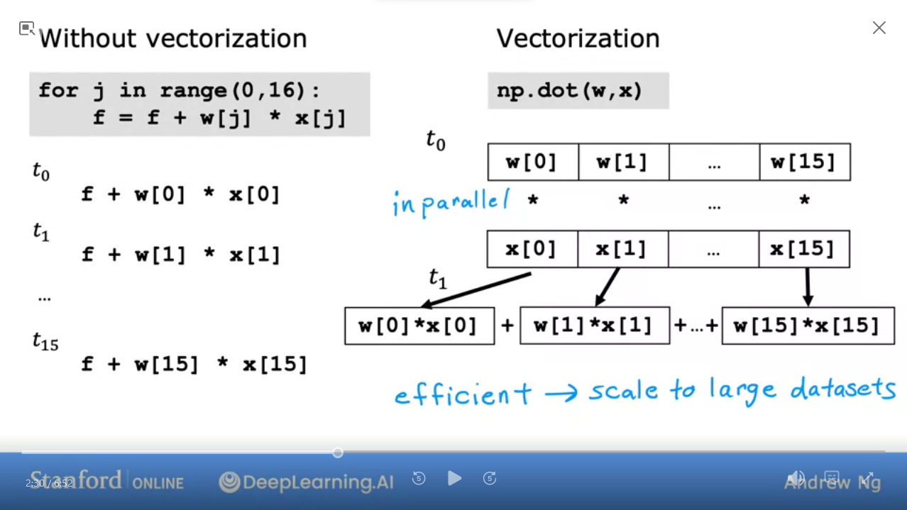
- Without vectorization, we run calculations linearly
-
np.dotworks in multiple steps:- get values of the vectors
w, x - In parallel run
w[i] * x[i]
- get values of the vectors

C1_W2_Lab01: Python Numpy Vectorization
C1_W2_M1_4 Gradient descent for multiple linear regression
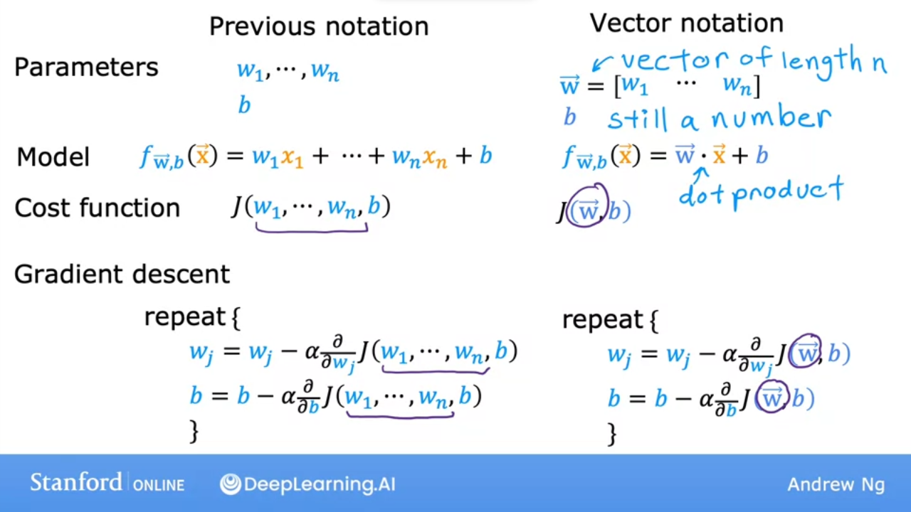

-
w & xare now vectors - have to update all the parameters simultaneously for$w_{1} .. w_{n}$as well as$b $

- Normal Equation
C1_W2_Lab02: Muliple linear regression
-
[Optional Lab: Multiple linear regression Coursera](https://www.coursera.org/learn/machine-learning/ungradedLab/7GEJh/optional-lab-multiple-linear-regression/lab) - Local
Quiz: Multiple linear regression
- In the training set below, what is$x_4^{(3)} $?
| Size | Rooms | Floors | Age | Price |
|---|---|---|---|---|
| 2104 | 5 | 1 | 45 | 460 |
| 1416 | 3 | 2 | 40 | 232 |
| 1534 | 3 | 2 | 30 | 315 |
| 852 | 2 | 1 | 36 | 178 |
- Which of the following are potential benefits of vectorization?
- It makes your code run faster
- It makes your code shorter
- It allows your code to run more easily on parallel compute hardware
- All of the above
- To make a gradient descent converge about twice as fast, a technique that almost always works is to double the learning rate$alpha $
- True
- False
Ans
30, 4, FC1_W2_M2 Gradient Descent in Practice
C1_W2_M2_01 Feature scaling part 1
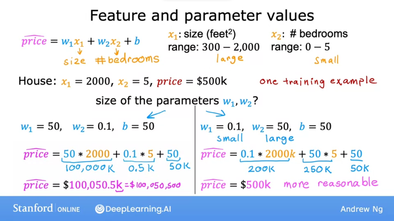
- Use Feature Scaling to enable gradient descent to run faster
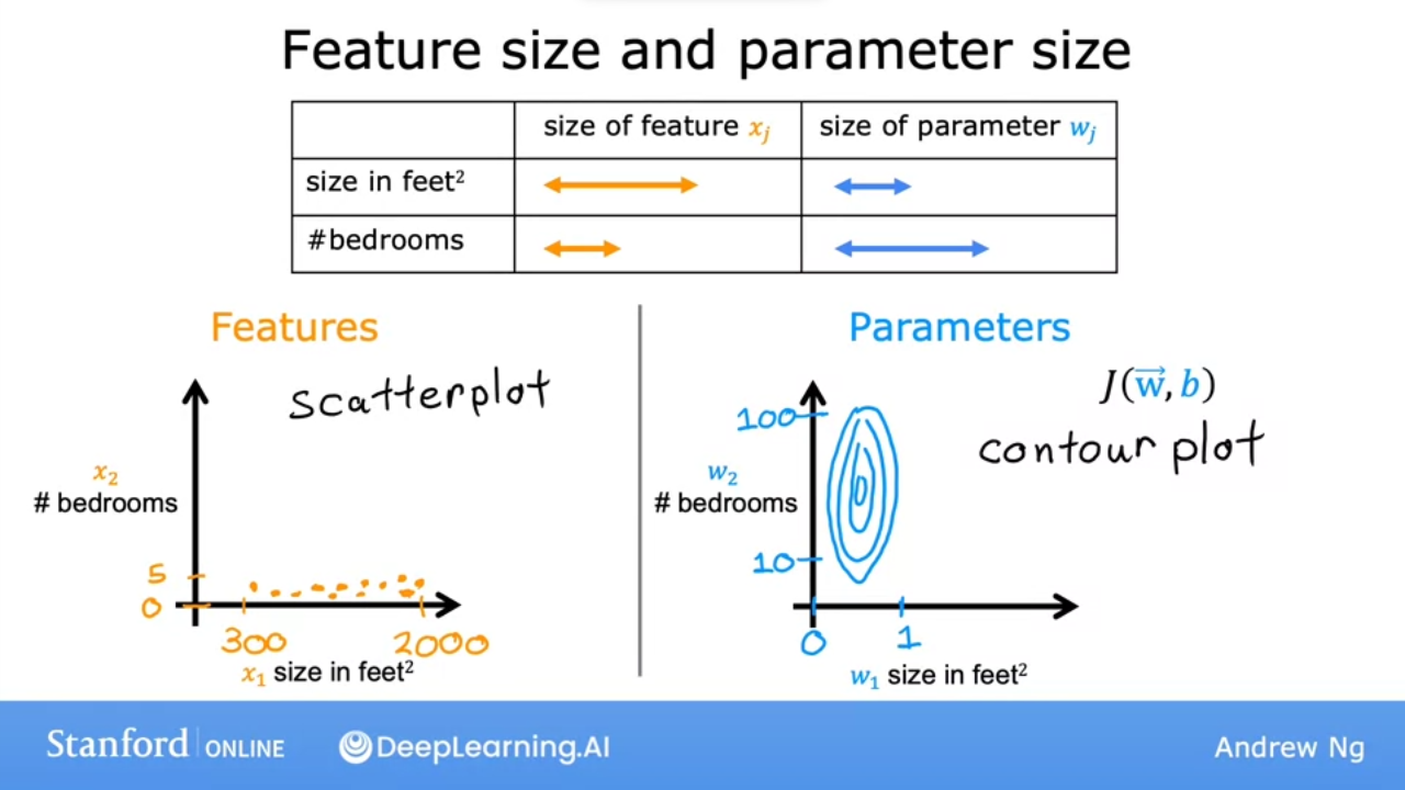
- when we scatterplot size vs bedrooms, we see
xhas a much larger range thany - when we contour plot we see an oval
- ie small
w(size)has a large change & largew(bedroomshas a small change
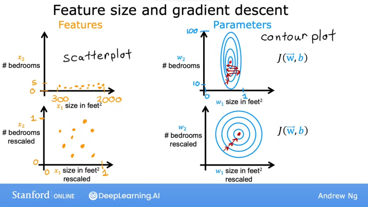
- since contour is tall & skinny, gradeient descent may end up bouncing back and forth for a long time
- a technique is to scale the data to get a more circular contour plot
![]() We can speed up gradient descent by scaling our features
We can speed up gradient descent by scaling our features
C1_W2_M2_02 Feature scaling part 2
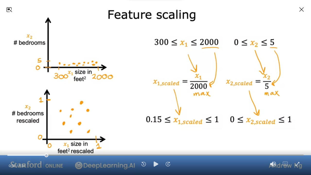
- scale by dividing$x_i^{(j)} / \max_x $
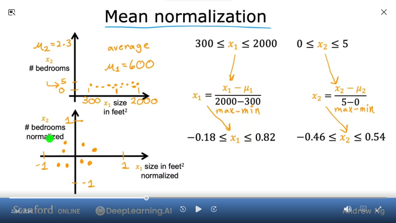
- Mean Normalization
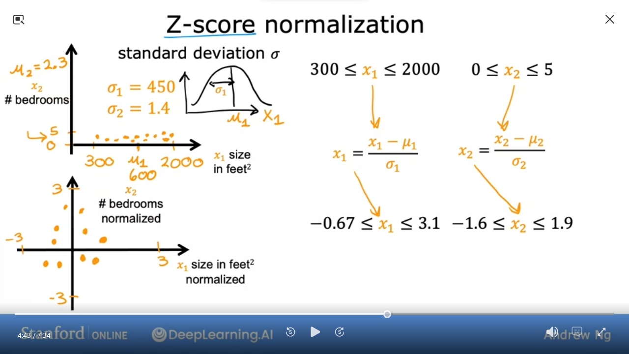
- Z-score Normalization also called Gaussian Distribution
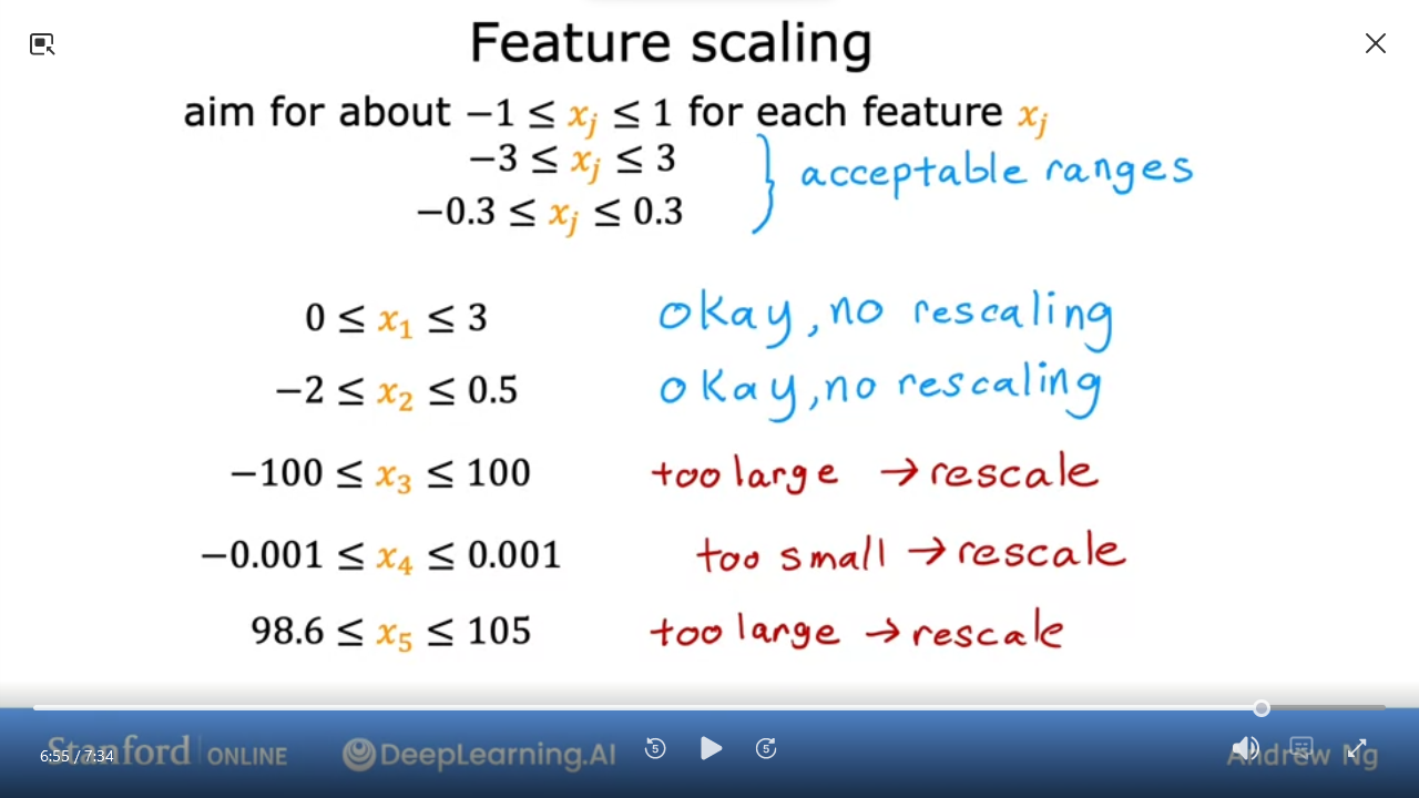
- When Feature Scaling we want to range somewhere between
-1 <==> 1 - but the range is ok if it’s relatively close
- rescale if range is too large or too small
Quiz:
Which of the following is a valid step used during feature scaling? (see bedrooms vs size scatterplot)
- Multiply each value by the maximum value for that feature
- Divide each value by the maximum value for that feature
Ans
2C1_W2_M2_03 Checking gradient descent for convergence

- We can choose$\alpha $

- Want to minimize cost function $\min\limits_{\vec{w}, b} J(\vec{w}, b)$
C1_W2_M2_04 Choosing the learning rate
C1_W2_M2_05 Optional Lab: Feature scaling and learning rate
C1_W2_M2_06 Feature engineering
C1_W2_M2_07 Polynomial regression
C1_W2_M2_08 Optional lab: Feature engineering and Polynomial regression
C1_W2_M2_09 Optional lab: Linear regression with scikit-learn
C1_W2_M2_10 Practice quiz: Gradient descent in practice
C1_W2_M2_11 Week 2 practice lab: Linear regression

