Supervised vs Unsupervised Machine Learning
1 What is machine learning?
Field of study that gives computers the ability learn without being explicitly pogrammed – Arthur Samuel
2 Supervised Learning: Regression Algorithms
#Supervised_Learning Given inputs x, predict output y
| Input (x) | Output (Y) | Application |
|---|---|---|
| spam? (0/1) | spam filtering | |
| audio | text transcripts | speech recognition |
| English | Spanish | machine translation |
| ad, user | click? (0/1) | online advertising |
| image, radar | position of other cars | self-driving car |
| image of phone | defect? (0/1) | visual inspection |
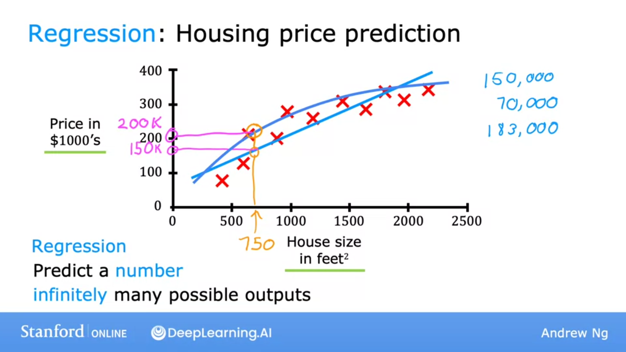
- We can use different algorithms to predict price of house based on data
3 Supervised Learning: Classification
- #Regression attempts to predict infinite possible results
- #Classification predicts categories ie from limited possible results
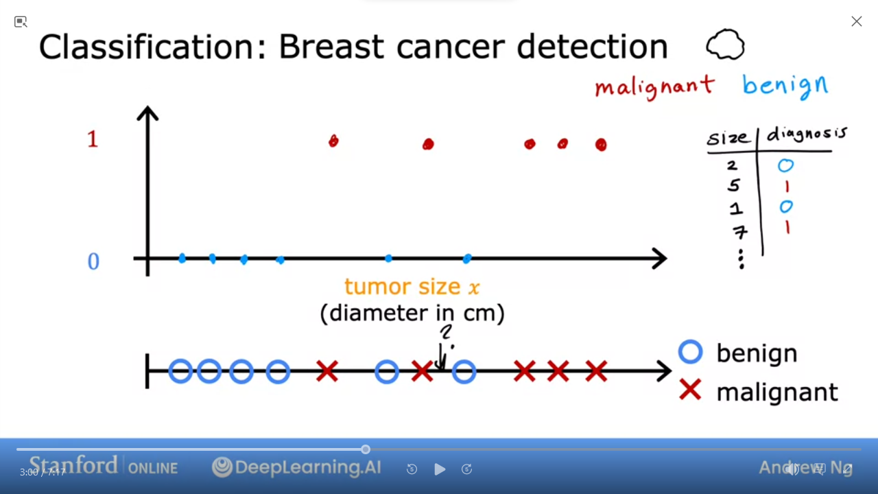
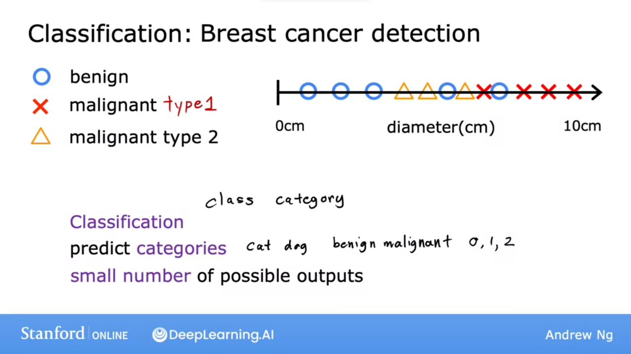
- we can have multiple outputs
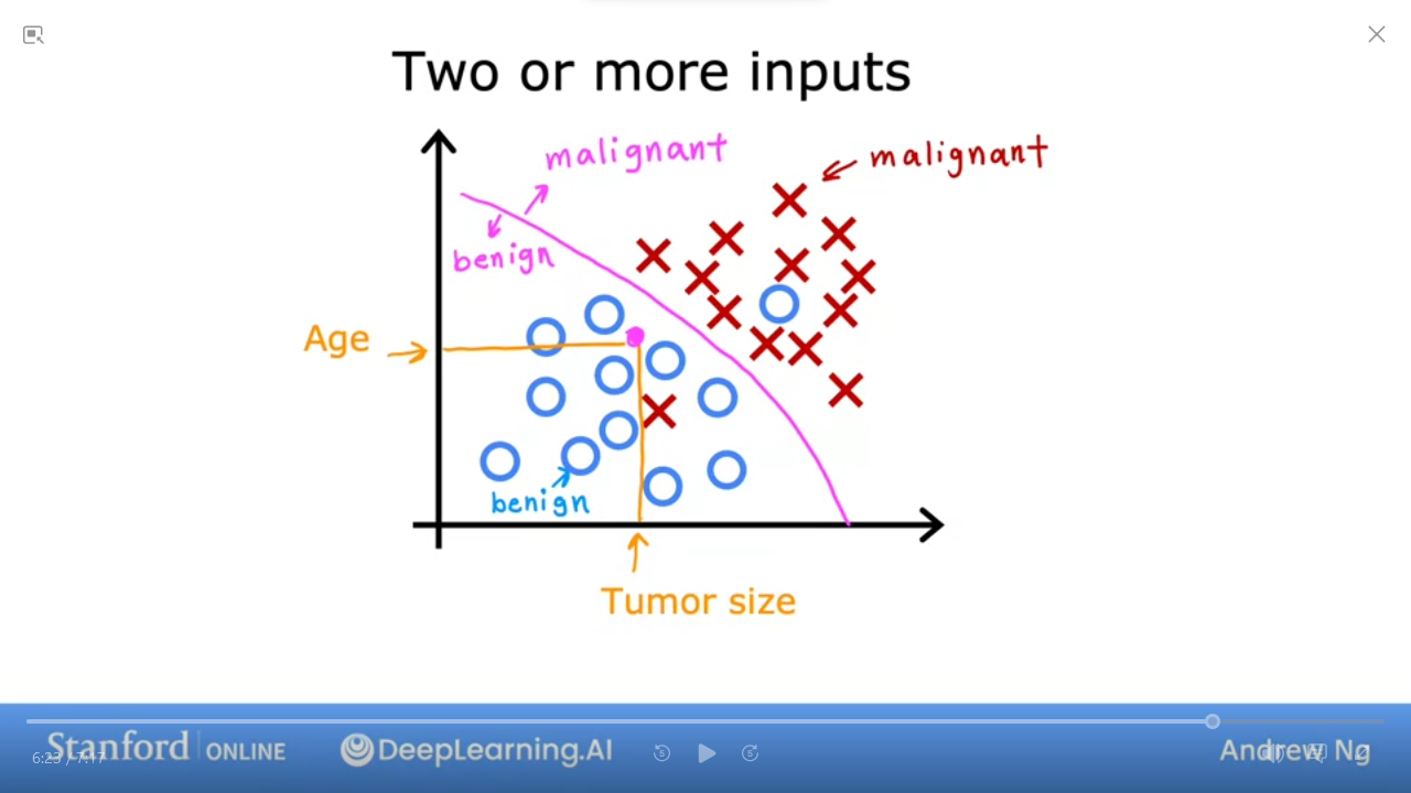
- we can draw a boundary line to separate our output
| Regression | Classification | |
|---|---|---|
| Predicts | numbers | categories |
| Outputs | infinite | limited |
4 Unsupervised Learning: Clustering, Anomaly Detection
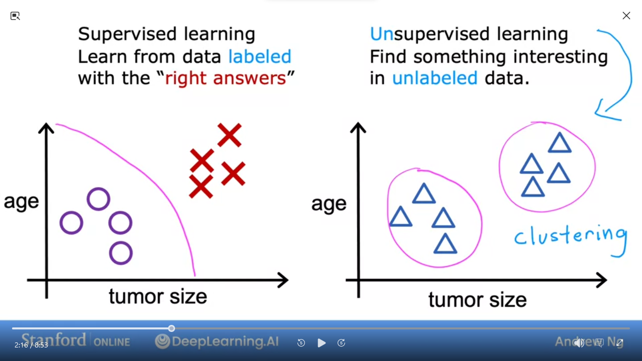
- With unsupervised we don’t have predetermined expected output
- we’re trying to find structure in the pattern, in this example clustering
- e.g. Google News will “cluster” news related to pandas given a specific article about panda/birth/twin/zoo
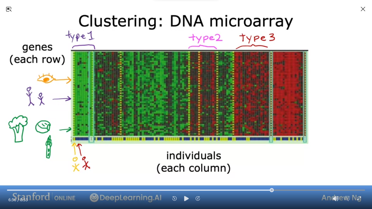
- e.g. given set of individual genes, cluster similar genes
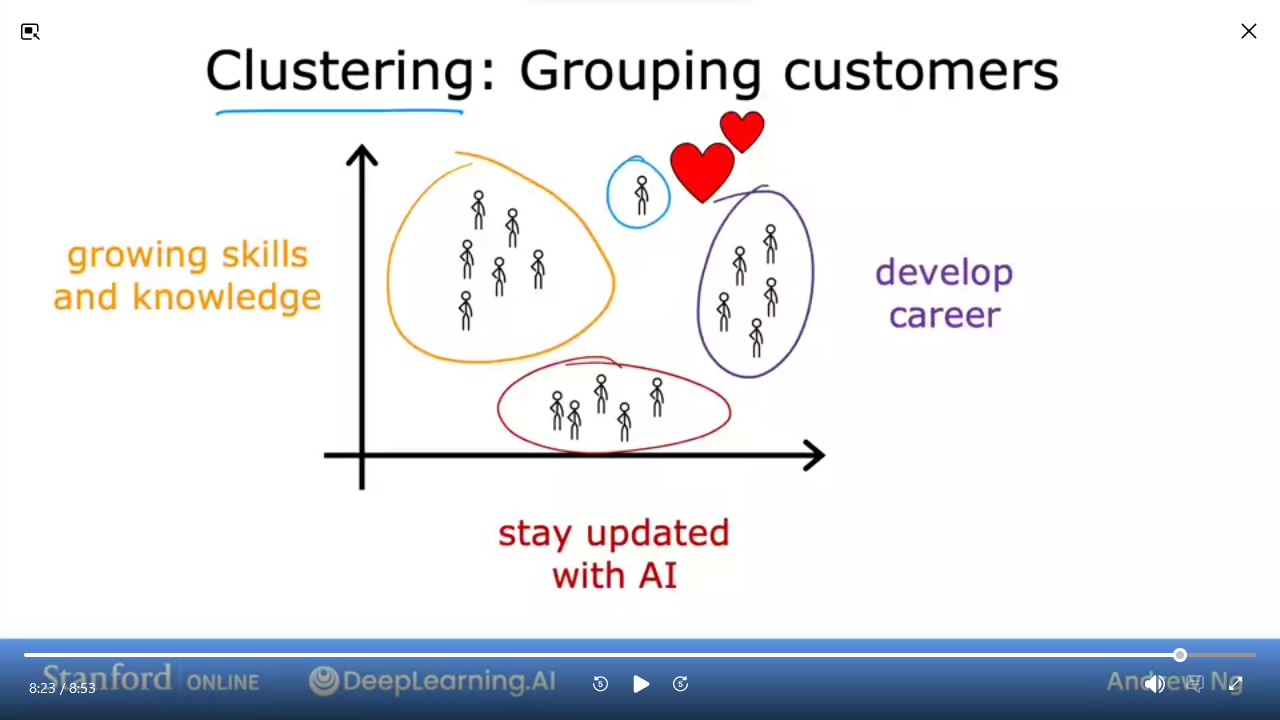
- e.g. how deeplearning.ai categorizes their learners
#Unsupervised_Learning Data only comes with inputs x, but not output labels y. Algorithm has to find structure in the data
- #Clustering Group similar data points together
- #Anomaly_Detection Find unusual data points
- #Dimensionality_Reduction Compress data using fewer numbers
Question:
Of the following examples, which would you address using an unsupervised learning algorithm?
(Check all that apply.)
- Given a set of news articles found on the web, group them into sets of articles about the same stories.
- Given email labeled as spam/not spam, learn a spam filter.
- Given a database of customer data, automatically discover market segments and group customers into different market segments.
- Given a dataset of patients diagnosed as either having diabetes or not, learn to classify new patients as having diabetes or not.
Ans
1,3Lab 01: Python and Jupyter Notebooks
Learn basics of Jupyter Local: Jupyter Notebook || Coursera Jupyter
Quiz: Supervised vs Unsupervised Learning
Which are the two common types of supervised learning (choose two)
- Classification
- Regression
- Clustering
Which of these is a type of unsupervised learning?
- Clustering
- Regression
- Classification
Ans
- 1,2 - 1Regression Model
1 Linear Regression Model
#Linear_Regression_Model => a Supervised Learning Model that simply puts a line through a dataset
- most commonly used model
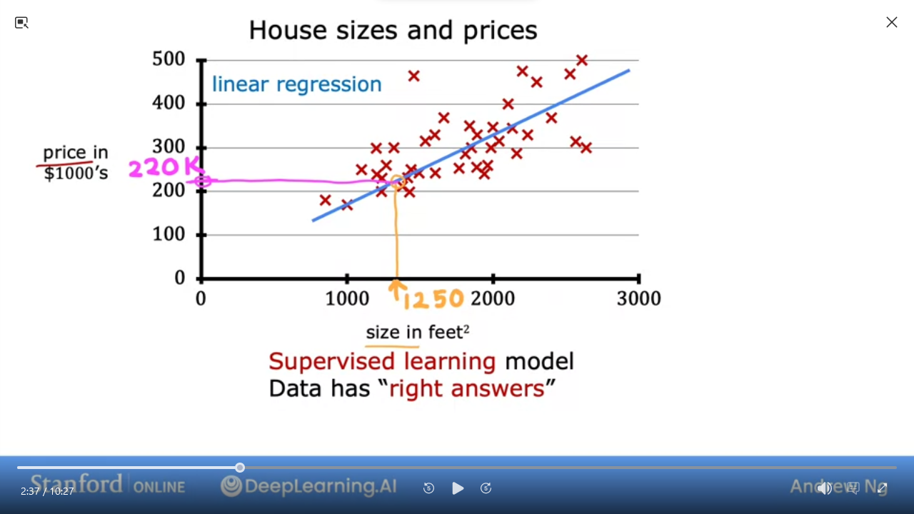
- e.g. Finding the right house price based on dataset of houses by sq ft.
| Terminology | |
| ———–: | :————————— |
| Training Set | data used to train the model |
| x | input or #feature |
| y | output variable or #target |
| m | number of training examples |
| (x,y) | single training example |
| (xⁱ,yⁱ) | i-th training example |
f is a linear function with one variable
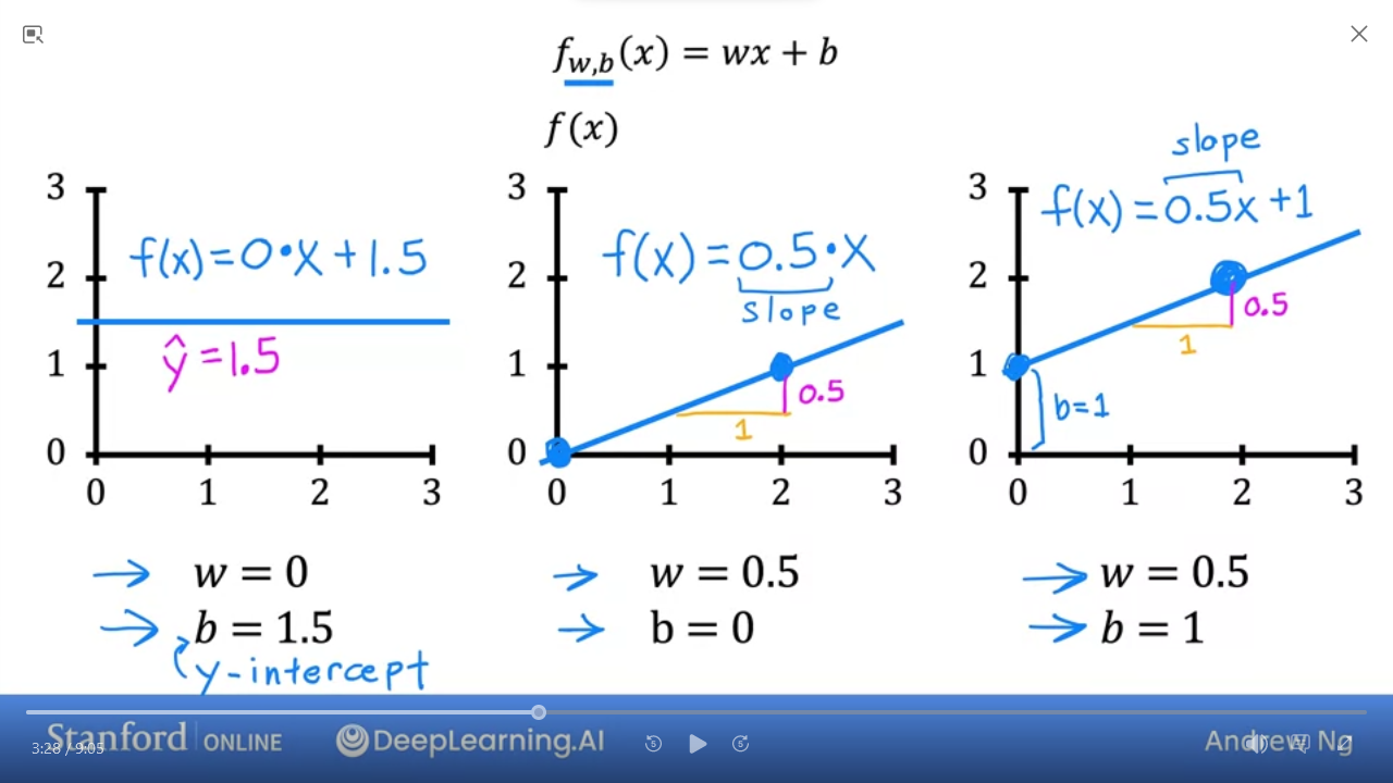
- $f_{w,b}(x) = wx + b$ is equivalent to
- $f(x) = wx + b$
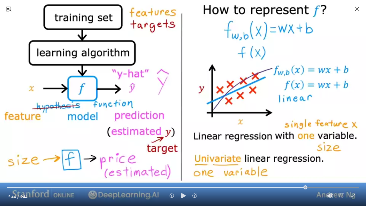
- Univariate linear regression => one variable
Lab 02: Model representation
Coursera Jupyter: Model representation || Local Jupyter
In this lab you will learn: - Linear regression builds a model which establishes a relationship between features and targets
- In the example, the feature was house size and the target was house price
- For simple linear regression, the model has two parameters $w$ and $b$ whose values are fit using training data.
- Once a model’s parameters have been determined, the model can be used to make predictions on novel data.
| | Python | Description |
| :—————— | :———- | :———————————————————————————————————————– |
| $\mathbf{x}$ | x_train | Training Example feature values (in this lab - Size (1000 sqft)) |
| $\mathbf{y}$ | y_train | Training Example targets (in this lab Price (1000s of dollars)) |
| $x^{(i)}$,$y^{(i)}$ | x_i,y_i | $i_{th}$Training Example |
| m | m | Number of training examples |
| $w$ | w | parameter: #weight (slope) |
| $b$ | b | parameter: #bias (y-intersect) |
| $f_{w,b}(x^{(i)})$ | f_wb | #Model_Function The result of the model evaluation at $x^{(i)}$ parameterized by w,b $f_{w,b}(x^{(i)}) = wx^{(i)}+b$ |
Code
NumPy, a popular library for scientific computingMatplotlib, a popular library for plotting datascatter()to plot on a graphmarkerfor symbol to usecfor color
Goal is to find the w, b to give you best fit line through your data
import numpy as np                       # https://numpy.org/ for mathematical calculations
import matplotlib.pyplot as plt          # https://matplotlib.org package for 2D graphs
plt.style.use('./deeplearning.mplstyle') # matplotlib style sheet

x_train = np.array([1.0, 2.0])      # x_train is the input (size in 1000 square feet)
y_train = np.array([300.0, 500.0])  # y_train is target (price in 1000s of dollars)

def compute_model_output(x, w, b):      # Computes the prediction of a linear model
  m = x_train.shape[0]                  # `.shape[0]` returns the number of rows
  f_wb = np.zeros(m)                    # return 1-dim array of zeros
  for i in range(m):
    f_wb[i] = w * x[i] + b              # compute the model output
  return f_wb

w = 200; b = 100;       # w = weight, b = bias; These are the params you can modify
tmp_f_wb = compute_model_output(x_train, w, b)

plt.plot(x_train, tmp_f_wb, c='blue',label='Our Prediction') # Plot our prediction
plt.scatter(x_train, y_train, marker='x', c='red',label='Actual Values')
plt.title("Housing Prices")                                  # Set the title
plt.ylabel('Price (in 1000s of dollars)')                    # Set the y-axis label
plt.xlabel('Size (1000 sqft)')                               # Set the x-axis label
plt.legend(); plt.show()
4 Cost function formula
- We can play with
w&bto find the best fit line
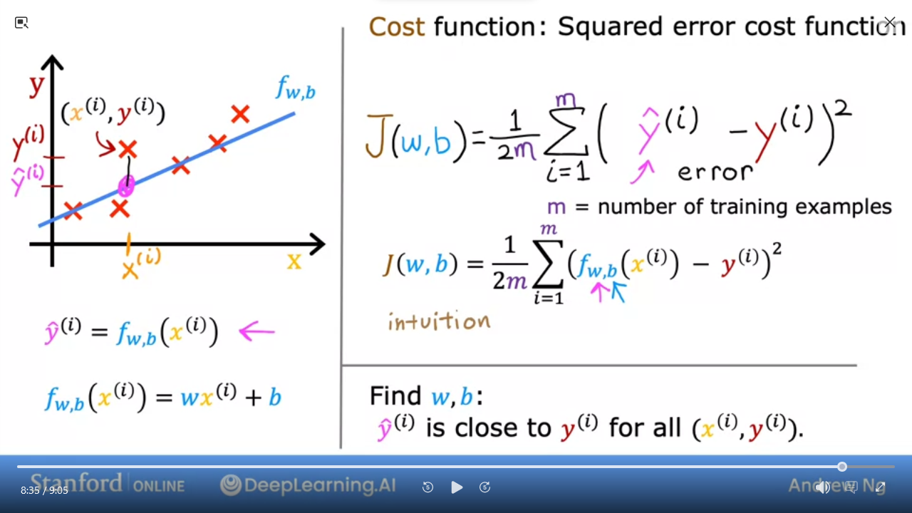
- #Cost_Function is a formula that measures the difference between predicted and actual values, aiming to minimize the error between them. It serves as a performance metric for evaluating a model’s fitness .
- 1st step to_implement linear function is to define Cost_Function
- Given $f_{w,b}(x) = wx + b$ where
wis the #slope andbis the #y-intercept Cost functiontakes predicted $\hat{y}$ and compares toy- ie
error= $\hat{y} - y$ - $\sum\limits_{i=1}^{m} (\hat{y}^{(i)} - y^{(i)})^{2}$ where
mis the number of training examples - Dividing by
2mmakes the calculation neater $\frac{1}{2m} \sum\limits_{i=1}^{m} (\hat{y}^{(i)} - y^{(i)})^{2}$ - Also known as #squared_error_cost_function $J_{(w,b)} = \frac{1}{2m} \sum\limits_{i=1}^{m} (\hat{y}^{(i)} - y^{(i)})^{2}$
- Which can be rewritten as $J_{(w,b)} = \frac{1}{2m} \sum\limits_{i=1}^{m} (f_{w,b}(x^{(i)}) - y^{(i)})^{2}$
- Remember we want to find values of
w,bwhere $\hat{y}^{(i)}$ is close to $y^{(i)}$ for all $(x^{(i)}, y^{(i)})$
Question:
Which of these parameters of the model that can be adjusted? -$w$ and $b$ -$f_{w,b}$ -$w$ only, because we should choose $b = 0$ -$\hat{y}$
Ans
15 Cost Function Intuition
To get a sense of how to minimize $J$ we can use a simplified model
| simplified | ||
|---|---|---|
| model | $f_{w,b}(x) = wx + b$ | $f_{w}(x) = wx$ by setting $b=0$ |
| parameters | $w, b$ | $w$ |
| cost function | $J_{(w,b)} = \frac{1}{2m} \sum\limits_{i=1}^{m} (f_{w,b}(x^{(i)}) - y^{(i)})^{2}$ | $J_{(w)} = \frac{1}{2m} \sum\limits_{i=1}^{m} (f_{w}(x^{(i)}) - y^{(i)})^{2}$ |
| goal | we want to minimize$J_{(w,b)}$ | we want to minimize$J_{(w)}$ |
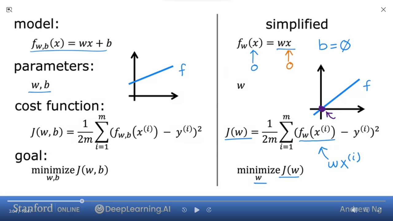
- we can use simplified function to find the best fit line
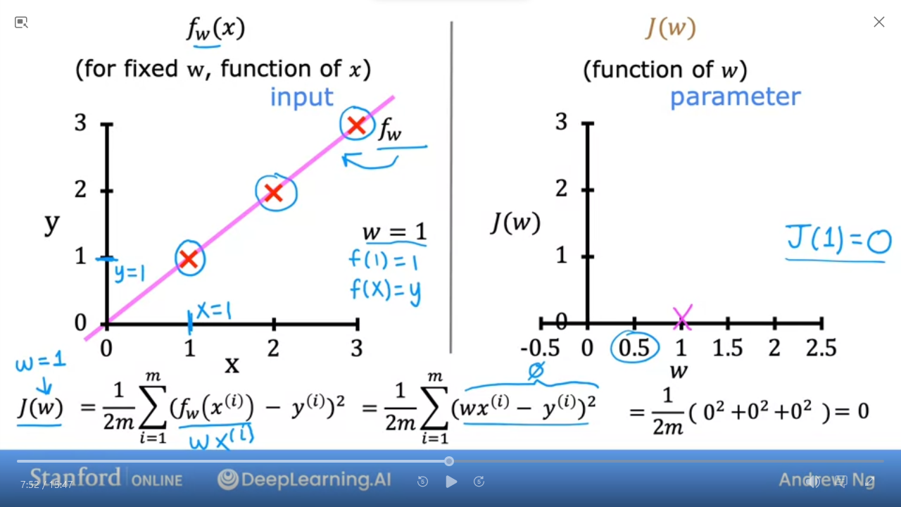
- the 2nd graph shows that when $w = 1$ then $J(1) = 0$
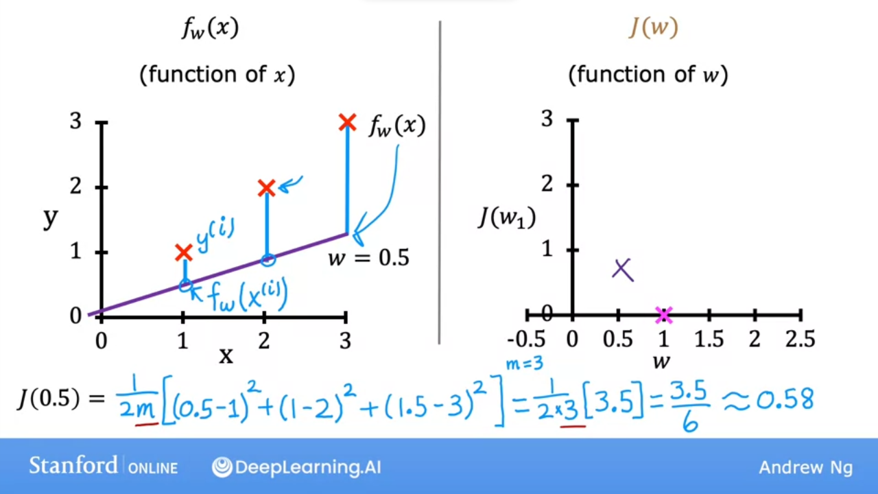
- the 2nd graph shows that when $w = 0.5$ then $J(0.5) ~= 0.58$
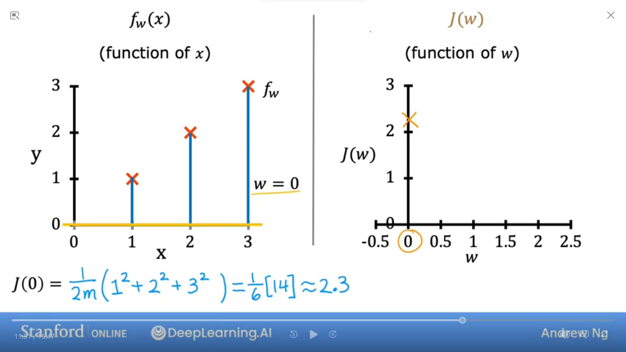
- the 2nd graph shows that when $w = 0$ then $J(0) \approx 2.33$
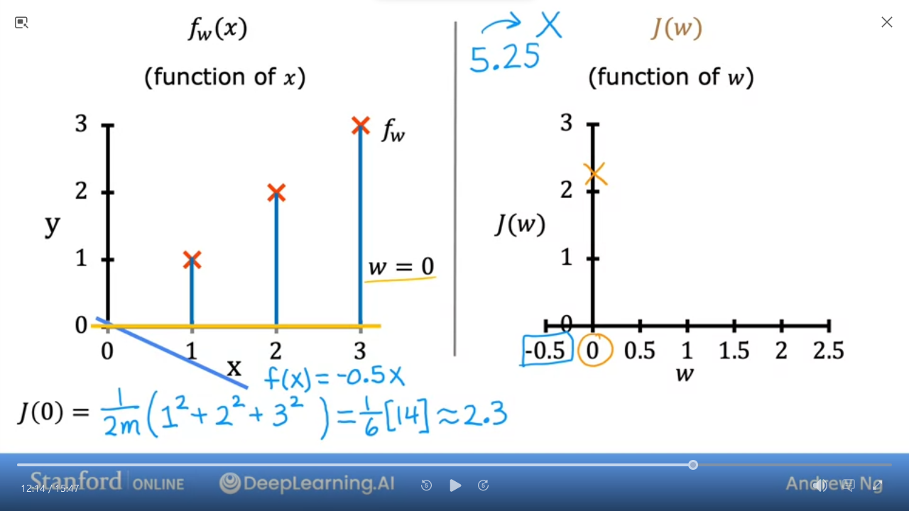
- We can do this calculation for various $w$ even negative numbers
- when $w = -0.5$ then $J(-0.5) \approx 5.25$
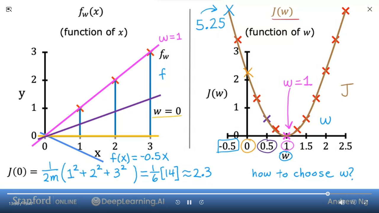
- We can plot various values for
wand get a graph (on the right) - As we can see the cost function with $w = 1$ is the best fit line for this data
💡 The goal of linear regression is to find the values of $w,b$ that allows us to minimize $J_{(w,b)}$
6 Visualizing the cost function
| model | $f_{w,b}(x) = wx + b $``$ |
| parameters | $w$,$b$ |
| cost function | $J_{(w,b)} = \frac{1}{2m} \sum\limits_{i=1}^{m} (f_{w,b}(x^{(i)}) - y^{(i)})^{2}$ |
| goal | minimize $J_{(w,b)}$ |
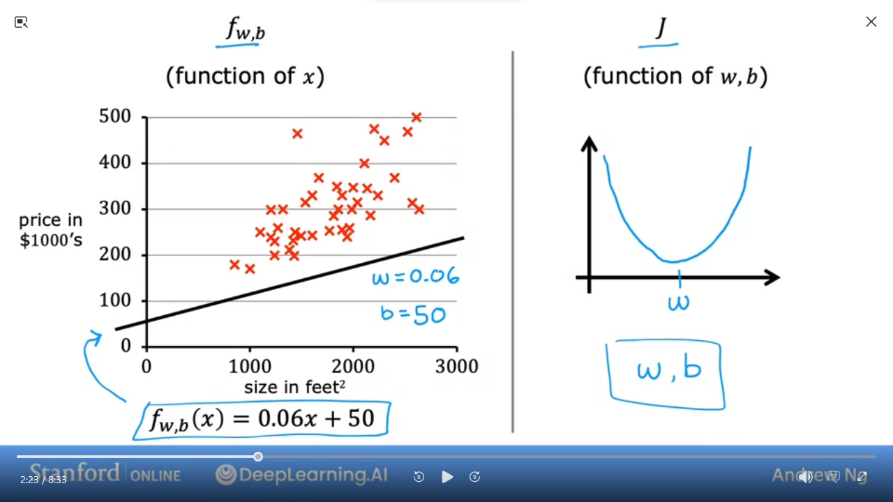
- When we only have w, then we can plot
Jvswin 2-dimensions
- However, when we add
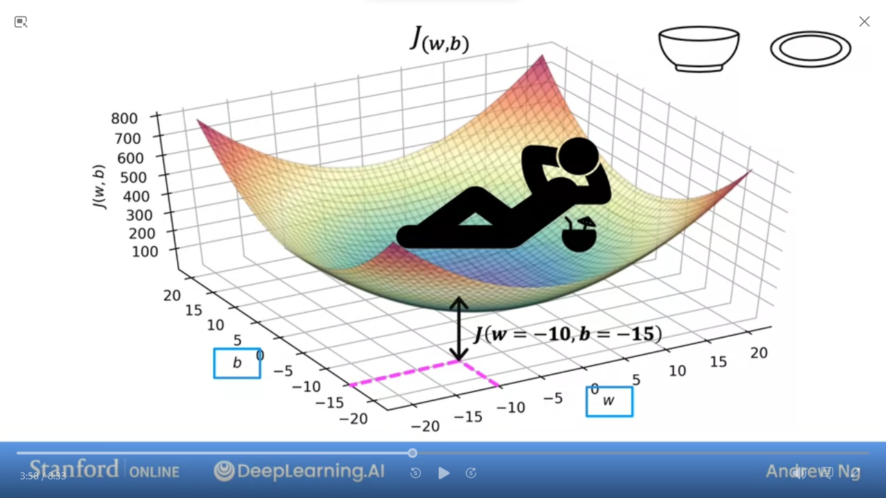
bthen it’s 3-dimensional - The value of
Jis the height
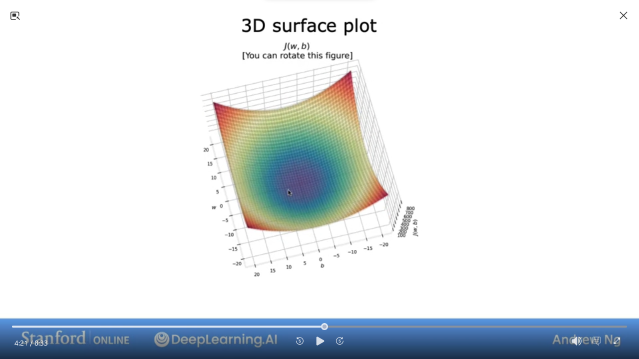
- this is easier to visualize as a
contour plot

- Same as used to visualize height of mountains
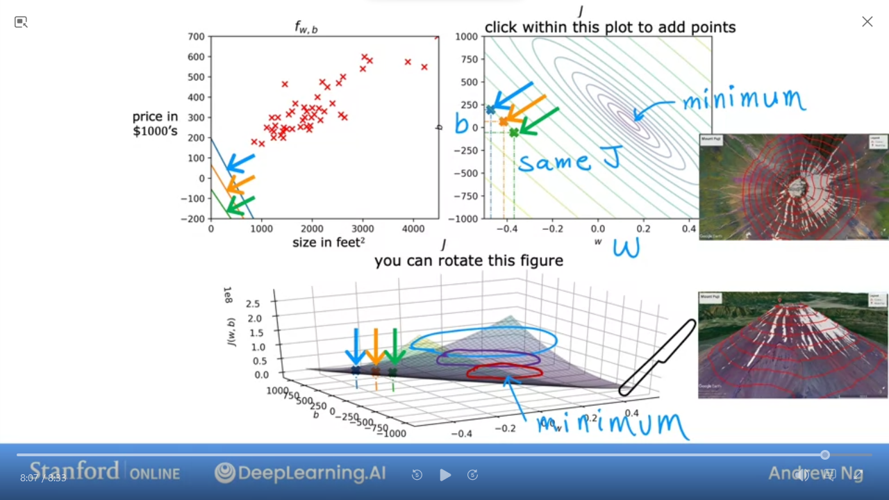
- take a horizontal slice which gives you the same
Jfor givenw,b - the center of the contour is the minimum
- #Countour allows us to visualize the 3-D
Jin 2-D
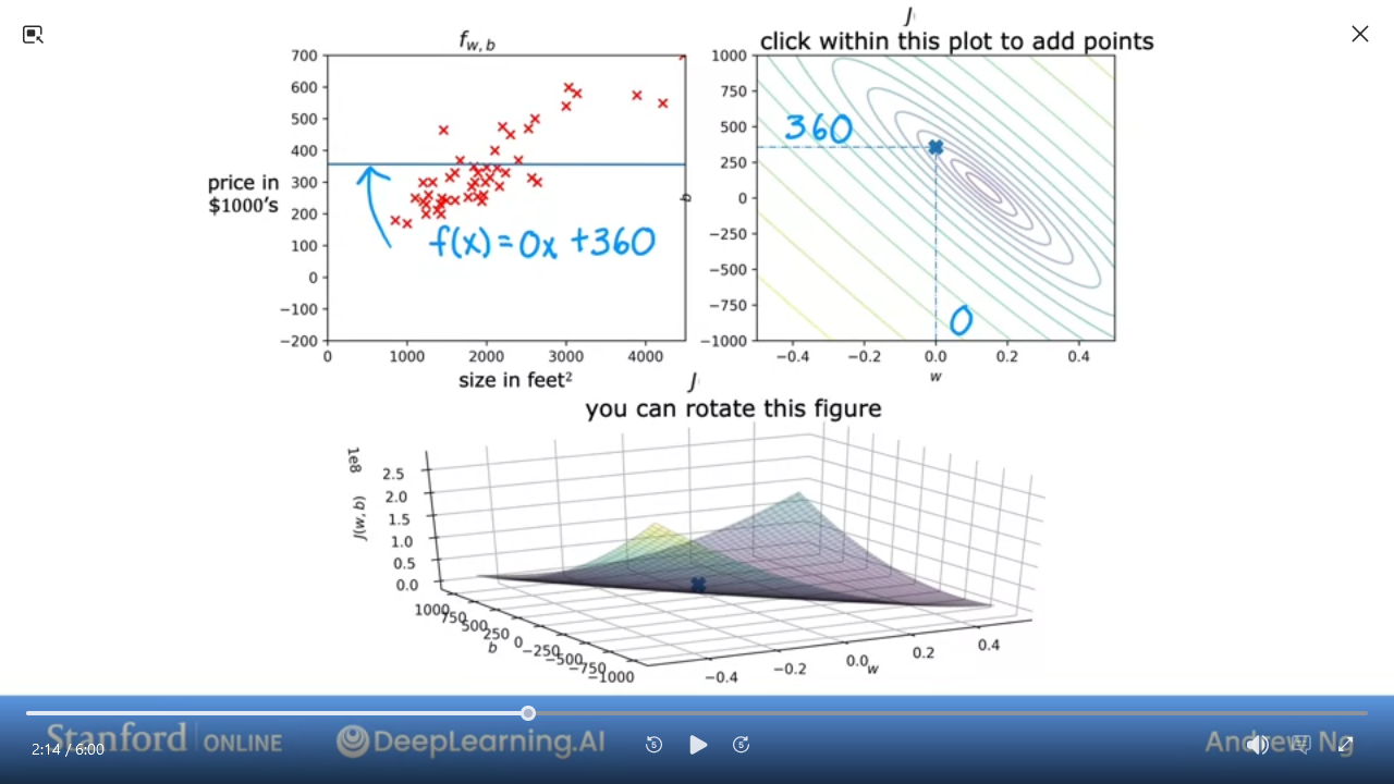
7 Visualization examples
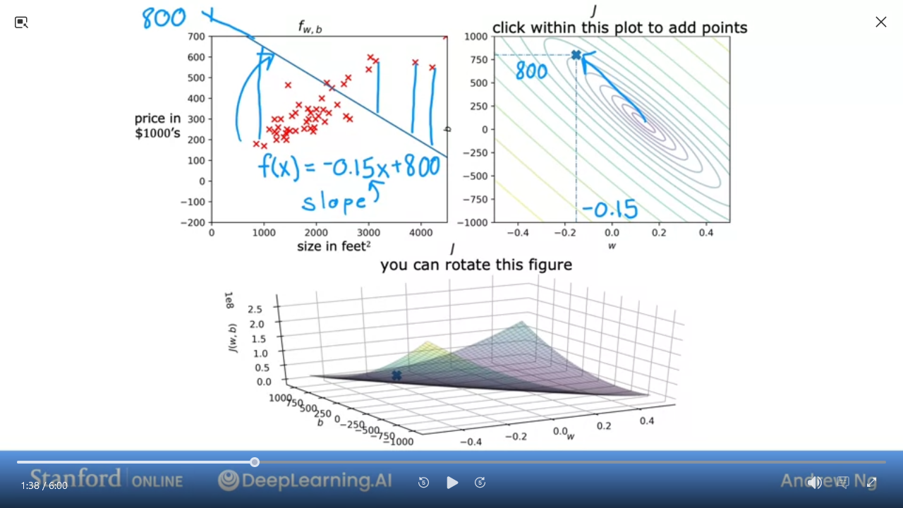
- We can see this is a pretty bad
J
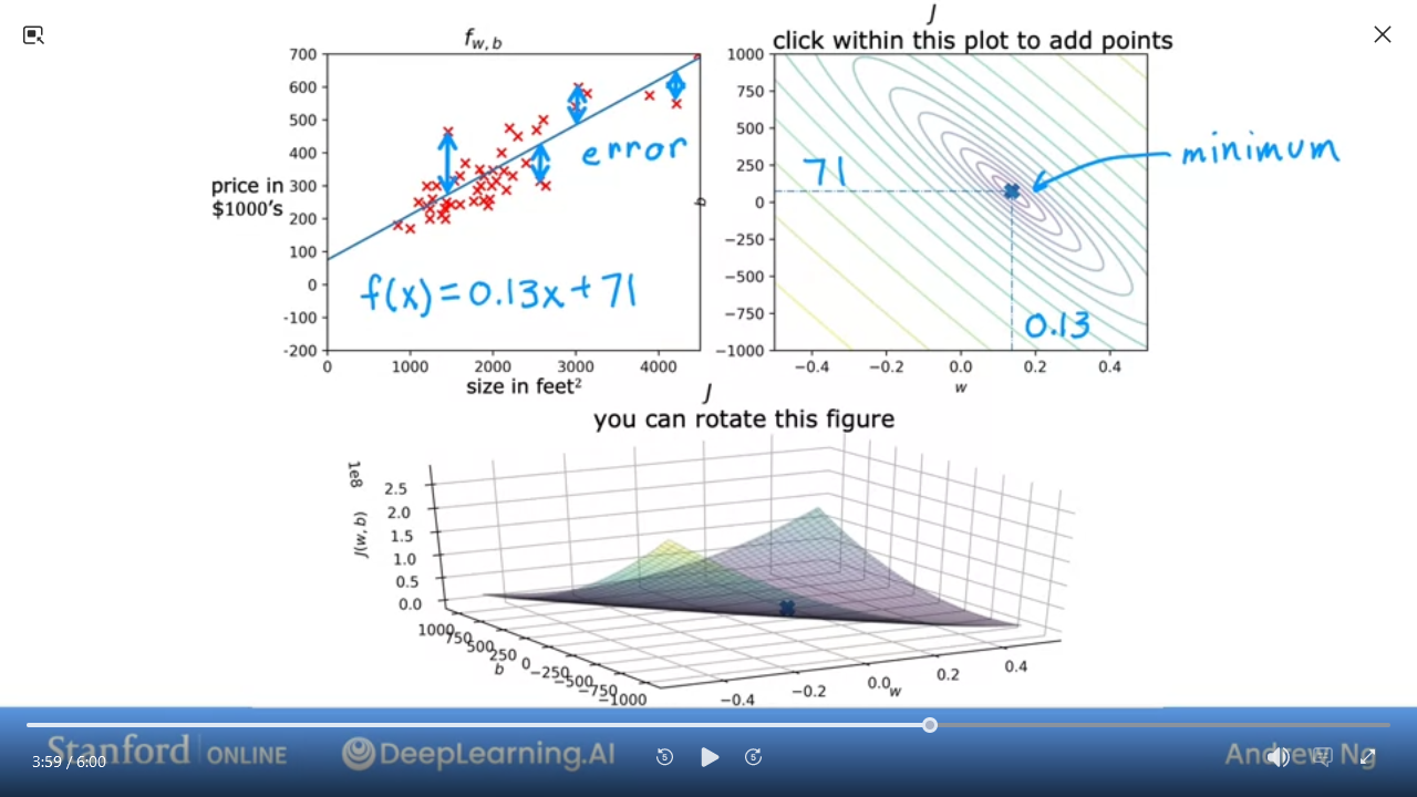
- This is pretty good and close to minimal (but not quite perfect)
In the next lab, you can click on different points on the contour to view the cost function on the graph
#Gradient_Descent is an algorithm to train linear regression and other complex models
Lab 03: Cost function
Coursera Jupyter: Cost Function || Local: Cost Function
- implement and explore the
costfunction for linear regression with one variable.# Cost Function cost_sum = 0 for i in range(m): f_wb = w * x[i] + b cost = (f_wb - y[i]) ** 2 cost_sum = cost_sum + cost total_cost = (1 / (2 * m)) * cost_sum
Quiz: Regression Model
- Which of the following are the inputs, or features, that are fed into the model and with which the model is expected to make a prediction?
- $m$
- $w$ and $b$
- $(x,y)$
- $x$
- For linear regression, if you find parameters $w$ and $b$ so that $J_{(w,b)}$ is very close to zero, what can you conclude?
- The selected values of the parameters $w, b$ cause the algorithm to fit the training set really well
- This is never possible. There must be a bug in the code
- The selected values of the parameters $w, b$ cause the algorithm to fit the training set really poorly
Ans
4, 1Train the model with gradient descent
1 Gradient descent
Want a systematic way to find values of $w,b$ that allows us to easily find smallest $J$
#Gradient_Descent is an algorithm used for any function, not just in linear regression but also in advanced neural network models
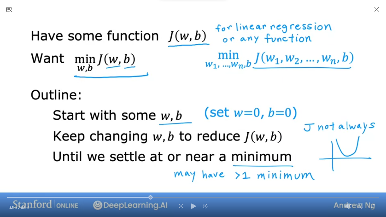
- start with some $w,b$ e.g. $(0,0)$
- keep changing $w,b$ to reduce $J(w,b)$
- until we settle at or near a minimum
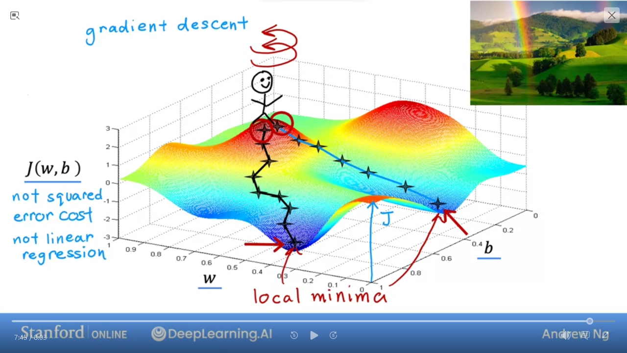
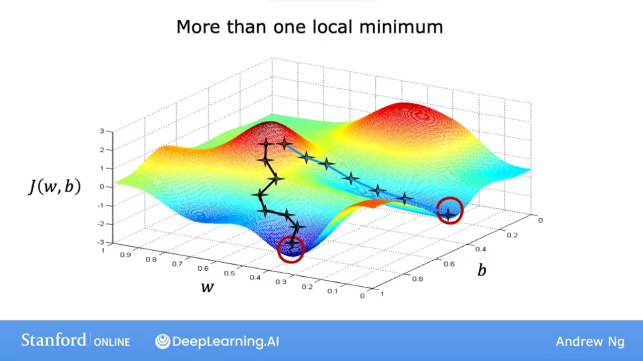
- Example of a more complex $J$ that is not a squared error cost nor linear regression
- we want to get to the lowest point in this topography
- pick a direction and take a step that is slightly lower, and repeat until you’re at lowest point
- However, depending on starting point and direction, you will end up at a different “lowest point”
- Known as #local_mimina
#local_minima may not be the true lowest point
2 Implementing gradient descent
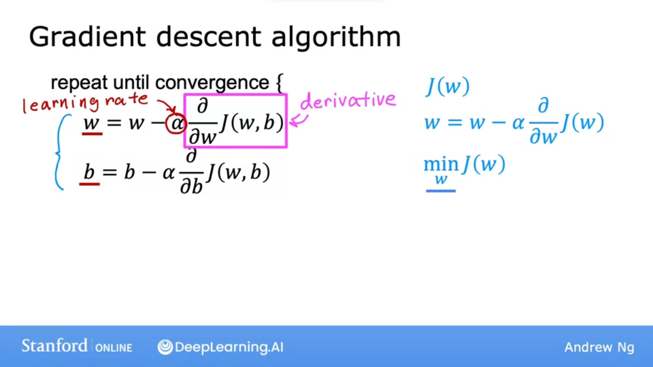
- The Gradient Descent algorithm
- $w = w - \alpha \frac{\partial}{\partial w} J_{(w,b)}$ -$\alpha$== #learning_rate ie How “big a step” you take down the hill -$\frac{\partial}{\partial w} J_{(w,b)}$== #derivative ie which direction -$b = b - \alpha \frac{\partial}{\partial b} J_{(w,b)}$
- We repeat these 2 steps for $w,b$ until the algorithm converges
- ie each subsequent step doesn’t change the value
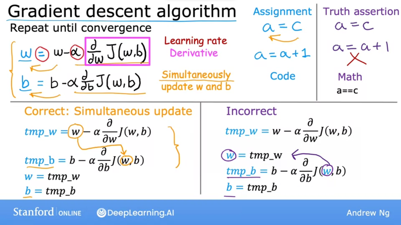
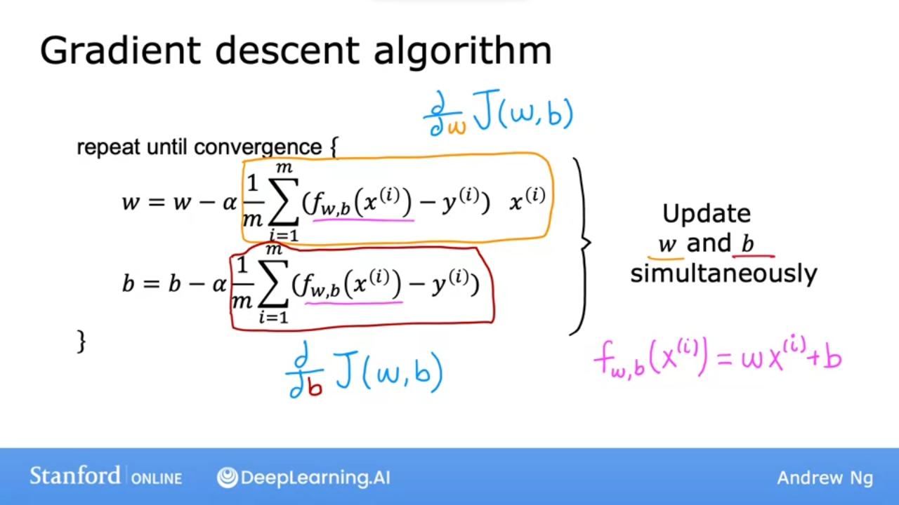
- We want to simultaneously update w and b at each step
tmp_w= $w - \alpha \frac{\partial}{\partial w} J_{(w,b)}$tmp_b= $b - \alpha \frac{\partial}{\partial b} J_{(w,b)}$w = tmp_w && b = tmp_b
3 Gradient descent intuition
- We want to find minimum
w,b
- Starting with finding
min wwe can simplify to just $J(w)$ - Gradient descent with $w = w - \alpha \frac{\partial}{\partial w} J_{(w)}$
- minimize cost by adjusting just
w: $\min J(w)$
- Recall previous example where we set
b = 0 - Initialize
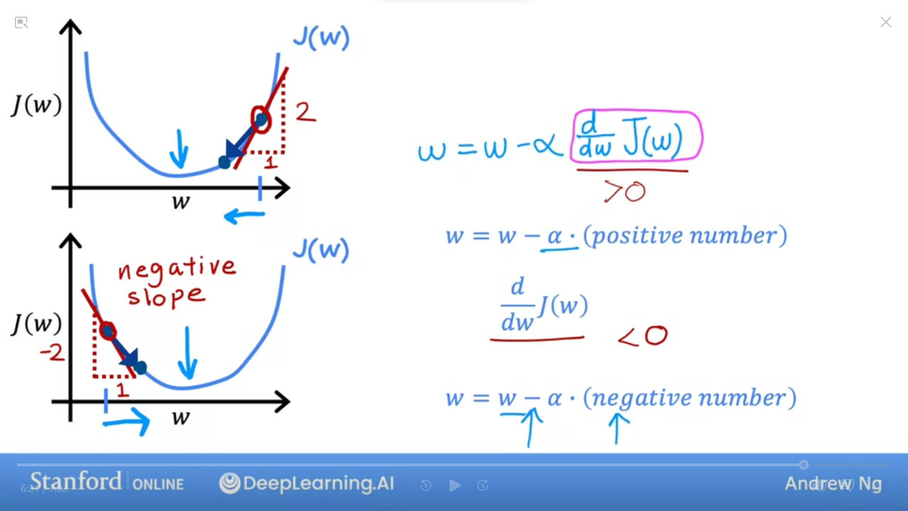
wat a random location - $\frac{\partial}{\partial w} J(w)$is the slope
- we want to find slopes that take us to minimum w
- In the first case, we get $w - \alpha (positive number)$ which is the correct direction
- However (2nd graph), slope is negative, and therefore also in the correct direction
4 Learning rate

- $\alpha$ is the learning rate ie how big a step to take
- If too small then you take small steps and will take a long time to find minimum
- If too big then you might miss true minimum ie diverge instead of converge
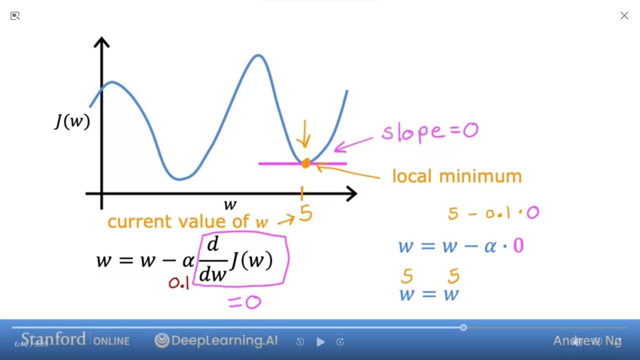
- If you’re already at local minimum…
slope = 0and therefore $\frac{\partial}{\partial w} J(w) = 0$- ie
w = w * 0 - further steps will bring you back here
- ie
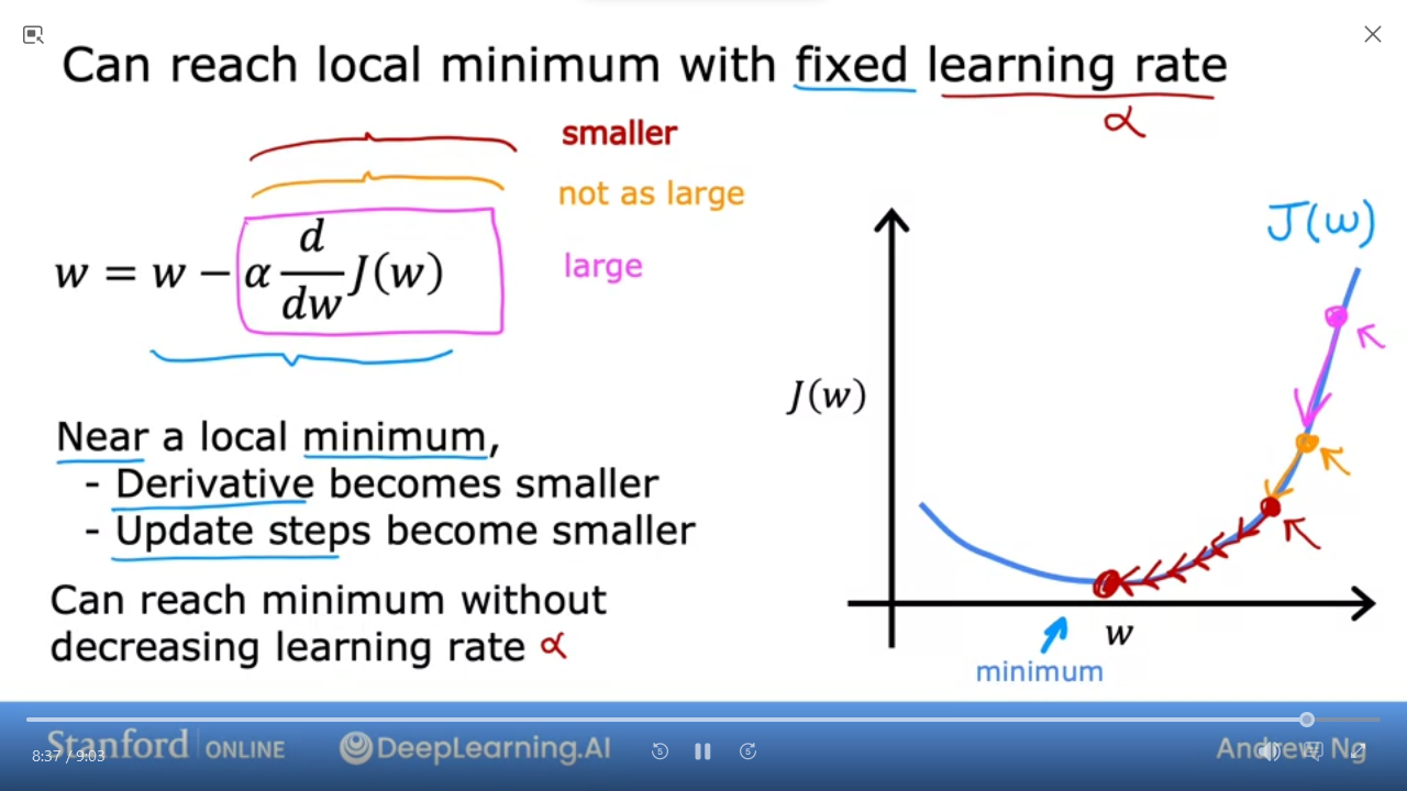
- As we get closer to local minimum, gradient descent (derivative function) will automatically take smaller steps
5 Gradient descent for linear regression
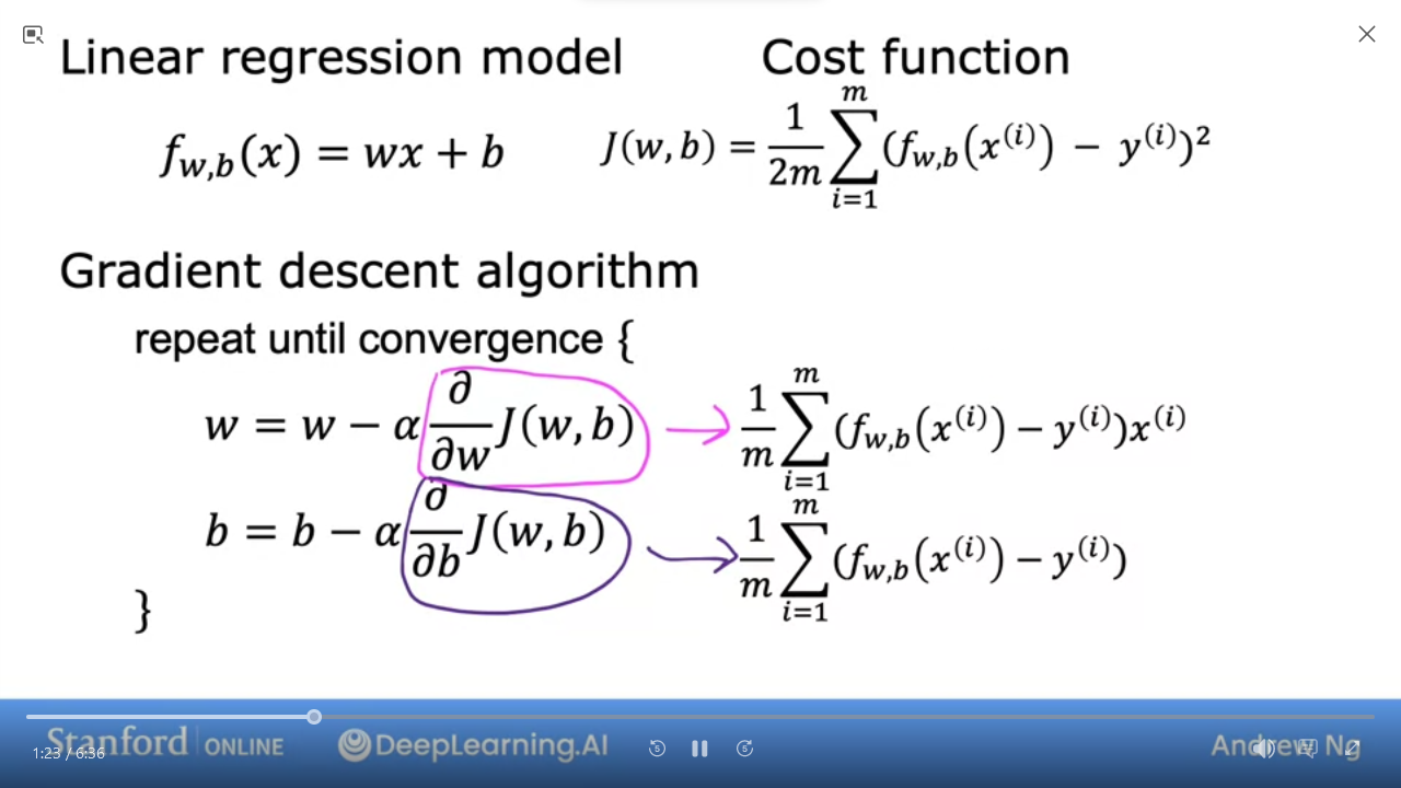
- #linear_regression_model $f_{w,b}(x) = wx + b$
- #cost_function $J_{(w,b)} = \frac{1}{2m} \sum\limits_{i=1}^{m} (f_{w,b}(x^{(i)} - y^{(i)})^{2}$
- #gradient_descent_algorithm
\(\begin{aligned} \text{repeat until convergence \{} \\ &w = w - \alpha \frac{\partial}{\partial w} J_{(w,b)}\\ &b = b - \alpha \frac{\partial}{\partial b} J_{(w,b)}\\ \} \end{aligned}\) - where $\frac{\partial}{\partial w} J_{(w,b)}$=$\frac{1}{m} \sum\limits_{i=1}^{m} (f_{w,b}(x^{(i)} - y^{(i)})x^{(i)}$
- and $\frac{\partial}{\partial b} J_{(w,b)}$=$\frac{1}{m} \sum\limits_{i=1}^{m} (f_{w,b}(x^{(i)} - y^{(i)})$
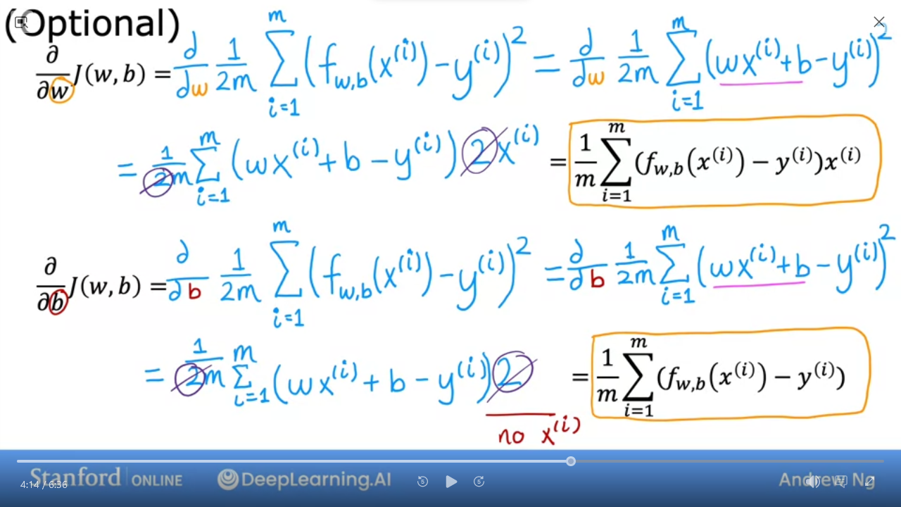
- We can simplify for
w
- and for
b
- a convex function will have a single global minimum
6 Running gradient descent
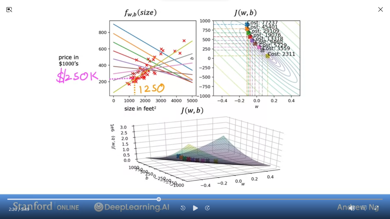
- left is plot of the model
- right is #contour_plot of the cost function
- bottom is the #surface_plot of the cost function
- for this example,
w = -0.1,b = 900 - as we take each step we get closer to the global minimum
- the yellow line is the best line fit
- Given a house with
1250 sq ft, we can predict it should sell for$250k per the model

- Batch Gradient Descent => each step of the gradient descent uses all the training examples
- DeepLearning.AI newsletter: The Batch
Lab 04: Gradient descent
Coursera Jupyter: Gradient descent || Local: Gradient Descent
- In this lab you:
- delved into the details of gradient descent for a single variable.
- developed a routine to compute the gradient
- visualized what the gradient is
- completed a gradient descent routine
- utilized gradient descent to find parameters
- examined the impact of sizing the learning rate
Quiz: Train the Model with Gradient Descent
- Gradient descent is an algorithm for finding values of parameters w and b that minimize the cost function $J$.
\(\begin{aligned}
\text{repeat until convergence \{} \\
&w = w - \alpha \frac{\partial}{\partial w} J_{(w,b)}\\
&b = b - \alpha \frac{\partial}{\partial b} J_{(w,b)}\\
\}
\end{aligned}\)
testing codeWhen $\frac{\partial}{\partial w} J_{(w,b)}$ is a negative number, what happens towafter one update step?- It is not possible to tell is
wwill increase or decrease - w increases
- w stays the same
- w decreases
- It is not possible to tell is
- For linear regression, what is the update step for parameter b?
- $b = b - \alpha \frac{1}{m} \sum\limits_{i=1}^{m} ((f_{w,b}(x^{(i)}) - y^{(i)})$
- $b = b - \alpha \frac{1}{m} \sum\limits_{i=1}^{m} ((f_{w,b}(x^{(i)}) - y^{(i)}) x^{(i)}$